曲线参数化
对于给定\(\mathbb{R}^2\)内一组有序点\(\{\mathbf{P}_i=(x_i,y_i)\}_{i=1}^n\),找到一组合适的实数\(\{t_i\}_{i=1}^n\),使得\(t_i\)与点\(\mathbf{P}_i\)一一对应。
下面是几种常用的曲线参数化算法:
均匀参数化 \[t_{i+1}-t_i=C\qquad (C\text{是常数})\]
弦长参数化 \[t_{i+1}-t_i=\Vert\mathbf{P}_{i+1}-\mathbf{P}_i\Vert_2\]
中心参数化 \[t_{i+1}-t_i=\sqrt{\Vert\mathbf{P}_{i+1}-\mathbf{P}_i\Vert_2}\]
Foley-Nielsen参数化 \[\begin{equation} t_{i+1}-t_i=\left\{ \begin{array}{ll} d_i\left[1+\frac{3\hat{\alpha}_{i+1}d_{i+1}}{2(d_i+d_{i+1})}\right] & i=1\\ d_i\left[1+\frac{3\hat{\alpha}_{i}d_{i-1}}{2(d_{i-1}+d_{i})}+\frac{3\hat{\alpha}_{i+1}d_{i+1}}{2(d_i+d_{i+1})}\right] & i=2,3\dots,n-2\\ d_i\left[1+\frac{3\hat{\alpha}_{i}d_{i-1}}{2(d_{i-1}+d_{i})}\right] & i=n-1 \end{array} \right. \end{equation}\] \[d_i=\Vert\mathbf{P}_{i+1}-\mathbf{P}_i\Vert_2\qquad \alpha_i=angle(\mathbf{P}_{i-1},\mathbf{P}_i,\mathbf{P}_{i+1})\qquad \hat{\alpha}_i=\min\left\{\alpha_i,\frac{\pi}{2}\right\}\]
拟合参数曲线
对于给定\(\mathbb{R}^2\)内一组点\(\{\mathbf{P}_i=(x_i,y_i)\}_{i=1}^n\),找到一个拟合这组点的向量值函数\(\mathbf{P}=f(t): \mathbb{R}\mapsto\mathbb{R}^2\),使得\(f(t)\)的轨迹尽可能靠近这组点。
拉格朗日型参数曲线拟合
\[\begin{equation} \left[ \begin{array}{c} x\\y \end{array}=f(t)=\left[ \begin{array}{c} a_0\\b_0 \end{array} \right]+\left[ \begin{array}{c} a_1\\b_1 \end{array} \right]t+\left[ \begin{array}{c} a_2\\b_2 \end{array} \right]t^2+\dots+\left[ \begin{array}{c} a_{n-1}\\b_{n-1} \end{array} \right]t^{n-1} \right] \end{equation}\] 将\(\{t_i,\mathbf{P}_i\}_{i=1}^n\)代入上式得到如下线性系统: \[\begin{equation} \left( \begin{array}{ccccc} 1&t_1&t_1^2&\cdots&t_1^{n-1}\\ 1&t_2&t_2^2&\cdots&t_2^{n-1}\\ \vdots&\vdots&\vdots&\ddots&\vdots\\ 1&t_n&t_n^2&\cdots&t_n^{n-1} \end{array} \right)\left( \begin{array}{cc} a_0&b_0\\ a_1&b_1\\ \vdots&\vdots\\ a_{n-1}&b_{n-1} \end{array} \right)=\left( \begin{array}{cc} x_1&y_1\\ x_2&y_2\\ \vdots&\vdots\\ x_n&y_n \end{array} \right) \end{equation}\] 通过求解上式线性系统可得到\(\mathbf{a}=[a_0,a_1,\dots,a_{n-1}]^{\mathsf{T}}\)和\(\mathbf{b}=[b_0,b_1,\dots,b_{n-1}]^{\mathsf{T}}\)。
高斯基函数型参数曲线拟合
\[\begin{equation} \left[ \begin{array}{c} x\\y \end{array}=f(t)=\left[ \begin{array}{c} a_0\\b_0 \end{array} \right]+\left[ \begin{array}{c} a_1\\b_1 \end{array} \right]g_1(t)+\left[ \begin{array}{c} a_2\\b_2 \end{array} \right]g_2(t)+\dots+\left[ \begin{array}{c} a_{n-1}\\b_{n-1} \end{array} \right]g_n(t) \right] \end{equation}\] 其中\(g_i(t)=exp(-(t-t_i)^2/(2\sigma^2))\),将\(\{t_i,\mathbf{P}_i\}_{i=1}^n\)代入上式可得到如下线性系统: \[\begin{equation} \left( \begin{array}{ccccc} 1&g_1(t_1)&g_2(t_1)&\cdots&g_n(t_1)\\ 1&g_1(t_2)&g_2(t_2)&\cdots&g_n(t_2)\\ \vdots&\vdots&\vdots&\ddots&\vdots\\ 1&g_1(t_n)&g_2(t_n)&\cdots&g_n(t_n) \end{array} \right)\left( \begin{array}{cc} a_0&b_0\\ a_1&b_1\\ \vdots&\vdots\\ a_{n-1}&b_{n-1} \end{array} \right)=\left( \begin{array}{cc} x_1&y_1\\ x_2&y_2\\ \vdots&\vdots\\ x_n&y_n \end{array} \right) \end{equation}\] 可以发现上式左边系数矩阵维数为\(n\times(n+1)\),未知数个数多余线性无关的方程个数,方程解不唯一。可添加单位1约束:\(\sum a_i=1\)和\(\sum b_i=1\)使得方程有唯一解,则得到如下方程: \[\begin{equation} \left( \begin{array}{ccccc} 1&g_1(t_1)&g_2(t_1)&\cdots&g_n(t_1)\\ 1&g_1(t_2)&g_2(t_2)&\cdots&g_n(t_2)\\ \vdots&\vdots&\vdots&\ddots&\vdots\\ 1&g_1(t_n)&g_2(t_n)&\cdots&g_n(t_n)\\ 1&1&1&\cdots&1 \end{array} \right)\left( \begin{array}{cc} a_0&b_0\\ a_1&b_1\\ \vdots&\vdots\\ a_{n-1}&b_{n-1} \end{array} \right)=\left( \begin{array}{cc} x_1&y_1\\ x_2&y_2\\ \vdots&\vdots\\ x_n&y_n\\ 1&1 \end{array} \right) \end{equation}\] 通过求解上式线性系统可得到\(\mathbf{a}=[a_0,a_1,\dots,a_{n-1}]^{\mathsf{T}}\)和\(\mathbf{b}=[b_0,b_1,\dots,b_{n-1}]^{\mathsf{T}}\)。
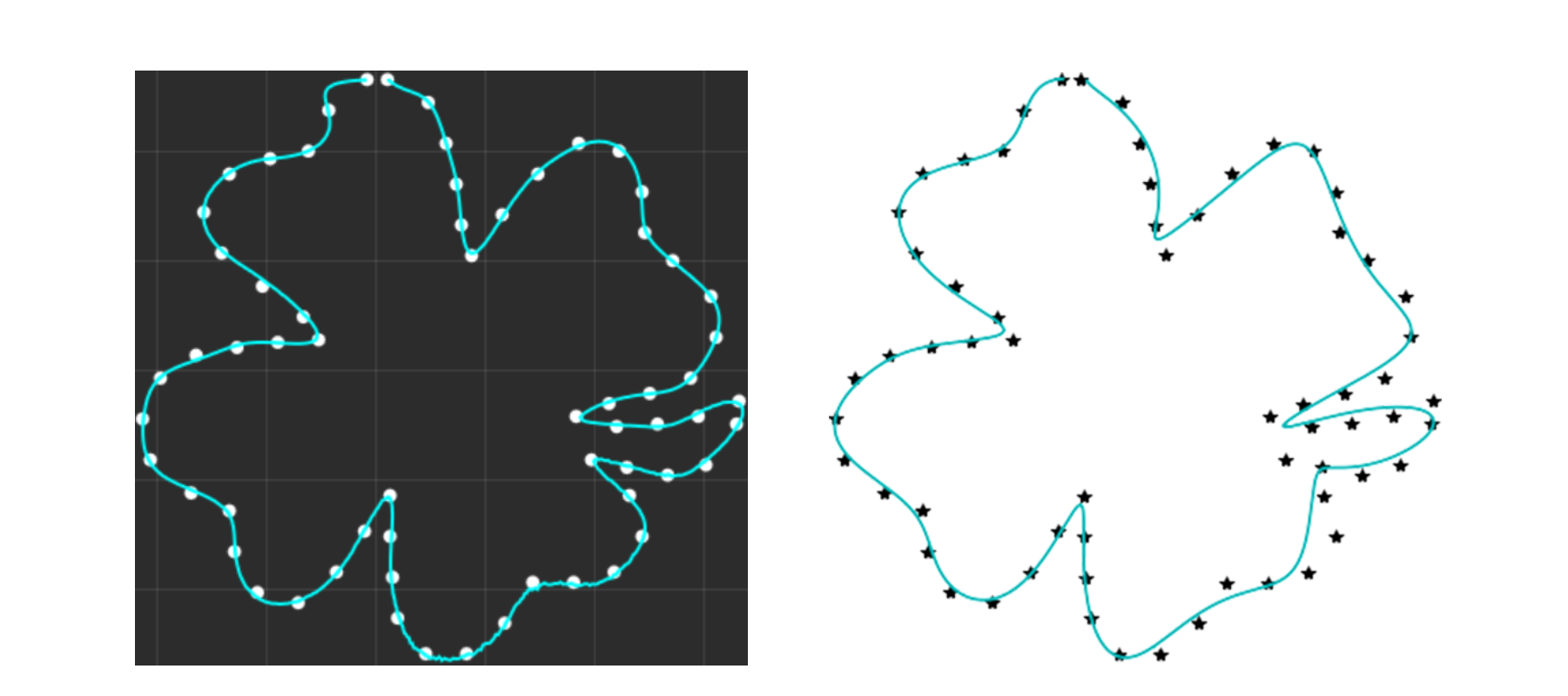
RBF算法拟合参数曲线
\[\begin{equation}
\left[
\begin{array}{c}
x\\y
\end{array}
\right]=f(t)=\left[
\begin{array}{c}
\omega_0+\sum_{i=1}^m\omega_ig_{0,1}(a_it+b_i)\\
\gamma_0+\sum_{i=1}^m\gamma_ig_{0,1}(\alpha_it+\beta_i)
\end{array}
\right]
\end{equation}\] 分别对上式中两个分量运用RBF算法,如下图所示 
最小二乘型参数曲线拟合
在拉格朗日型函数的基础上,考虑使用最高次数不高于\(m(m<n)\)的多项式作为基函数。 \[\begin{equation} \left[ \begin{array}{c} x\\y \end{array}=f(t)=\left[ \begin{array}{c} a_0\\b_0 \end{array} \right]+\left[ \begin{array}{c} a_1\\b_1 \end{array} \right]t+\left[ \begin{array}{c} a_2\\b_2 \end{array} \right]t^2+\dots+\left[ \begin{array}{c} a_{m}\\b_{m} \end{array} \right]t^m \right] \end{equation}\] 将\(\{t_i,\mathbf{P}_i\}_{i=1}^n\)代入上式可得到如下线性系统: \[\mathbf{AX}=\mathbf{P}\] 其中 \[\begin{equation} \mathbf{A}=\left( \begin{array}{ccccc} 1&t_1&t_1^2&\cdots&t_1^m\\ 1&t_2&t_2^2&\cdots&t_2^m\\ \vdots&\vdots&\vdots&\ddots&\vdots\\ 1&t_n&t_n^2&\cdots&t_n^m \end{array} \right)\qquad \mathbf{X}=\left( \begin{array}{cc} a_0&b_0\\ a_1&b_1\\ \vdots&\vdots\\ a_m&b_m \end{array} \right)\qquad\mathbf{P}=\left( \begin{array}{cc} x_1&y_1\\ x_2&y_2\\ \vdots&\vdots\\ x_n&y_n \end{array} \right) \end{equation}\] 通过对上式做最小二乘得到 \[(\mathbf{A}^{\mathsf{T}}\mathbf{A})\mathbf{X}=\mathbf{A}^{\mathsf{T}}\mathbf{P}\] 通过求解上式线性系统可得到\(\mathbf{a}=[a_0,a_1,\dots,a_{n-1}]^{\mathsf{T}}\)和\(\mathbf{b}=[b_0,b_1,\dots,b_{n-1}]^{\mathsf{T}}\)。
岭回归型参数曲线拟合
在最小二乘型拟合中添加正则约束,上式变为 \[(\mathbf{A}^{\mathsf{T}}\mathbf{A}+\lambda\mathbf{E})\mathbf{X}=\mathbf{A}^{\mathsf{T}}\mathbf{P}\] 通过求解上式线性系统可得到\(\mathbf{a}=[a_0,a_1,\dots,a_{n-1}]^{\mathsf{T}}\)和\(\mathbf{b}=[b_0,b_1,\dots,b_{n-1}]^{\mathsf{T}}\)。
数值试验
主要代码
均匀参数化
Eigen::VectorXf uniformParameterization(int numOfPoints) {
    Eigen::VectorXf y = Eigen::VectorXf::Zero(numOfPoints);
    for (int i=0; i<numOfPoints; ++i)
        y[i] = i;
    y /= y[numOfPoints -1]; return y;
}
弦长参数化
Eigen::VectorXf chordParameterization(std::vector<Ubpa::pointf2> points) {
    int n = points.size();
    Eigen::VectorXf y = Eigen::VectorXf::Zero(n);
    for (int i=1; i<n; ++i)
        y[i] = y[i-1]+(points[i]-points[i-1]).norm();
    y /= y[n-1];
    return y;
}
中心参数化
Eigen::VectorXf centripetalParameterization(std::vector<Ubpa::pointf2> points) {
    int n = points.size();
    Eigen::VectorXf y = Eigen::VectorXf::Zero(n);
    for (int i=1; i<n; ++i)
        y[i] = y[i-1]+sqrt((points[i]-points[i-1]).norm());
    y /= y[n-1];
    return y;
}
Foley-Nielsen参数化
Eigen::VectorXf FoleyParameterization(std::vector< Ubpa::pointf2> points) {
    int n = points.size();
    Eigen::VectorXf y = Eigen::VectorXf::Zero(n);
    if (n == 2) { y[1] = 1; return y; }
    Eigen::VectorXf dist = Eigen::VectorXf::Zero(n-1);
    Eigen::VectorXf alpha = Eigen::VectorXf::Zero(n-1);
    for (int i=0; i<n-1; ++i)
        dist[i] = (points[i+1]-points[i]).norm();
    for (int i=1; i<n-1; ++i) {
        float cosvalue = (points[i-1]-points[i]).cos_theta( points[i+1]- points[i]);
        alpha[i] = std::min(PI-acos(cosvalue), PI/2);
    }
    y[1] = dist[0]*(1+1.5*alpha[1]*dist[1]/(dist[0]+dist[1]));
    for (int i=2; i<n-1; ++i) {
        y[i] = y[i-1]+dist[i-1]*(1+1.5*alpha[i-1]*dist[i-2]/ (dist[i-2]+dist[i-1])+1.5*alpha[i]*dist[i]/ (dist[i-1]+dist[i]));
    }
    y[n-1] = y[n-2]+dist[n-2]*(1+1.5*alpha[n-2]*dist[n-3]/(dist[n-3]+dist[n-2]));
    y /= y[n-1];
    return y;
}
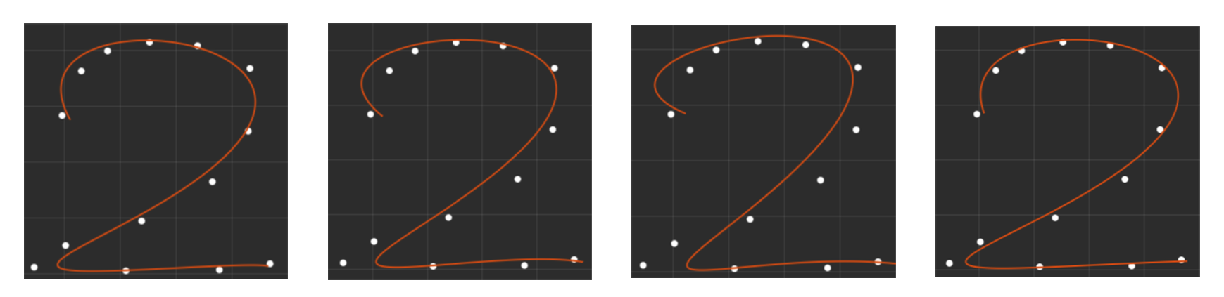
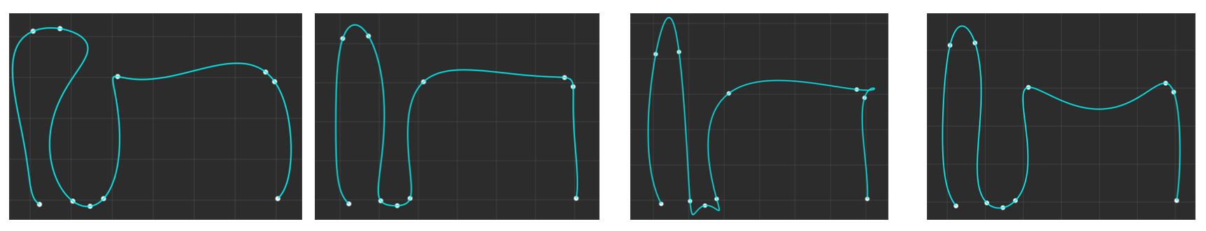
实验结果